
The feed forward neural nets work on the principle of predicting output at a given data point independently i.e. no dependency from past input. As there is no feedback from past, the network is not suitable for sequence modeling. Furthermore, the tasks where large data processing is involved requires Deep Neural Networks (DNN) and hence the term Deep Sequence Modeling
Sequential processing needs different neural network architecture. For example, an audio signal can be split into sequences of sound waves, text can be converted into sequence of characters or words, processing medical signals like EKGs, stock trend prediction and genomic data processing.
Consider building a language model where we need to predict the next word in the sentence say “Every night, I take my dog for a —– (walk)”. This task seems to be easy for humans but is way too complicated when the machine has to do it. Moreover, the automatic task carried out by the machine has reach human expectations or even higher than that. Let’s have a look at how we can kick start addressing the language model problem.
Issues and their solutions
Fixed Length Vector
The feed forward network if trained for such a task, can only process fixed length vectors whose length needs to be know before the processing begins. Sometimes, this is difficult to predict the length of the vector in advance as sentence may have variable word number.
We can still fix this issue by using a fixed window like, “for” =(10000)2, “a” = (01000)2 and using this one hot encoding scheme, we can predict the next work in the sequence.
Long Term Dependencies
The fixed window method has limitation of smaller history and hence long term dependencies cannot be modeled in the input data. For sentences such as “I spent my entire childhood in India, but I am working in Malaysia now. I can converse in —–”, (Hindi); the fixed window method won’t be able to hold on to the outlying past but only the recent past words based on window length.
Bag of words
Thus, we need a way to integrate information from across the sentence but also still represent the input as the fixed length vector. Another way we can do this is by actually using the entire sequence but representing it as a set of counts. This representation is called “Bag of Words”, where we can some vector and each slot in this vector represents a word and the value that’s in that slot represents the number of times that word appears in that sentence. Therefore, we have a fixed length vector of some vocabulary of words regardless of the length of input sentence but the counts are going to be different. We can feed this to feed-forward neural network and get the predicted next word.
This leads to another issue where maintaining the counts has completely abolished the entire sequence information. The sentences with different semantic meaning but same bag of words will have same counts. For instance, “The pink dress is showy and blue one is adorable” vs “the pink dress is adorable and the blue one is showy”.
Big fixed window
Consider, an example “This morning I ate bread and eggs on the table.” Now, when we train the NN with a larger window and if ever the start of the sentence appears in any other sentence at the end, the NN will find it difficult to recognize the next word as the parameters are not shared throughout the sentences.
Design requirements for Sequence Modeling
- Variable length sequences
- Long-term dependencies
- Sequence order
- Parameter sharing across sequences
Recurrent Neural Networks
To know why RNNs are preferred over conventional feed-forward neural network, we must know how RNN functions and also takes into account parameter sharing. For a more detailed functioning of RNN please refer to Introduction to Recurrent Neural Networks (RNN).
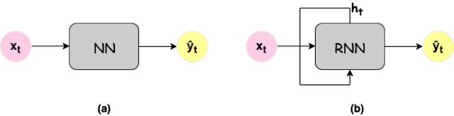
h_t = f_w (h_{t-1}, x_t)
where h_t = current cell state
Note: same functions and set of parameters are used at every time step
Output Vector
hat{y_t}= W_{hy} h_t
Hidden state : Update
h_t = tanh (W_{hh}h_{t-1}, W_{xh} x_t)
Why RNN?
- They take into account the first word x and compute its corresponding predicted output y’ , this is repeated till last time step. The number of input words are equal to number of output words.
- It scans data from left to right. Also the parameters are shared at every time step between input to hidden layer, hidden to hidden and hidden to output layer.
- Besides, we have information about say x_1 when we are making predictions for x_2 ie. access to past input when making predictions about current input. Incase, we need access to future inputs as well, we might use bi-directional RNN in place of the standard RNN.
The below figure shows the computational graph unwrapped across time during the forward and backward pass.

In Back Propagation Through Time (BPTT), the gradient or derivative of loss is computed against each parameter at every time time step and then finally summing the individual losses to calculate the over all loss L. The errors are back propagated at individual time steps and across time steps during the backward pass. While computing the loss function in a RNN, there are multiple matrix multiplications being carried out and also the derivative of the activation function computed. If these multiplication values are greater than unity, then the network experiences exploding gradients issue. This is rare phenomenon but easier to detect and correct. The gradient clipping can be employed to remove the bigger gradients. On the other hand, if the matrix values are too small, the network is likely to encounter vanishing gradients problem. This happens to be a major setback of the well known RNN. As a consequence, the network becomes unreliable in terms if long term dependencies.
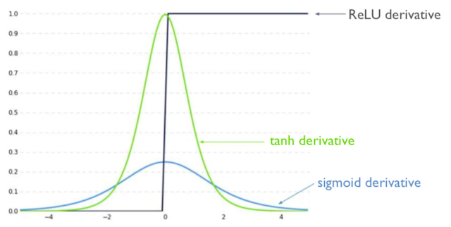
Overcome Vanishing Gradients
The product of the smaller values leads to shrinking of the number, ultimately reaching the zero line or vanishing. Further more, errors from the farer time steps are even more smaller. This implies that during the network training, we might end up biasing the parameters to get hold of the short–term dependencies. Hence, certain precautions during the start of training while designing the network architecture can prevent this undetectable catastrophic problem.
- Change of activation function: ReLu prevents the derivative of activation to fall to a smaller value.
- Initialization of weights: Setting the initial weights to identity matrix and all the biases to zero helps shrinking of gradients.
- Amendment in the RNN architecture: Use of gated cells like LSTM and GRU can control the vanishing gradient issue.
Long Short-Term Memory (LSTM)
The main aim of designing LSTMs is to store information in order to have long term dependencies. Hence, LSTMs are suitable for a variety of renowned applications such as speech recognition, machine translation and hand-writing recognition. The LSTMs employ gated activation function and maintain a special type of memory called cell state or state cell (in some references).
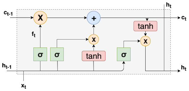
Gates: The gates perform the function of adding or removal of information. Optionally, gates let the data pass through a sigmoid function and pointwise multiplication.
Forget state: to forget unwanted part of previous state. It uses the previous cell input and output. Let f_t be the forget state at time t , g(.) is sigmoid activation function while b_f is the bias for forget state. When the sigmoid value is zero, the gate needs to forget the information completely at that time instant. On the other hand, when sigmoid value is unity, forget gates needs to keep the data intact.
f_t = g(W_j[h_{t-1},x_t]+b_f)
Update state: selectively updates cell state. As a part of update cell, firstly new information needs to be identified and then stored. This is useful incase of adding new feature to the processed data. Therefore, i_t be the information to be stored, and internal output cell state, tilde{C_t} ,
i_t = g(W_j[h_{t-1},x_t]+b_i)
tilde{C_t}=tanh(W_C[h_{t-1},x_t]+b_c)
The sigmoid layer helps to decide which value needs an update while the tanh layer contributes to adding vector of a new candidate. Consequently, the output of update cell is a sum of forget operation to previous internal cell state f_t*C_{t-1} and scaled new candidate value i_t * tilde{C_t} .
Output gate: selectively output parts of cell state. The sigmoid layer decides which parts of the state needs to be outputted while tanh scales values between -1 to +1 .
o_t =g(W_o[h_{t-1},x_t]+b_o)
h_t= o_t * tanh(C_t)
Please note all these multiplications are element wise. Matrix multiplications leads to vanishing gradient problem.